Parametric Exploration of the Mann-Whitney U Test 

Abraham Nunes MD PhD MBA 

Dalhousie University, Halifax, Nova Scotia, Canada 


The Binormal ROC Model and the U-Statistic 

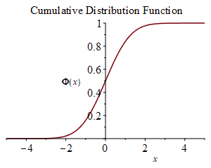
Recall that the CDF of a normal distribution is 

with(Statistics); -1 

Phi := proc (x) options operator, arrow, function_assign; CDF(Normal(0, 1), x) end proc; 1 

Typesetting:-mprintslash([Phi := proc (x) options operator, arrow, function_assign; Statistics:-CDF(Normal(0, 1), x) end proc], [proc (x) options operator, arrow, function_assign; Statistics:-CDF(Norm... (1.1)
 

plot(Phi(x), x = -5 .. 5, size = [.5, .8], labels = [x, 'Phi(x)'], title =  

Plot_2d
 

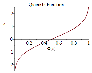
Q := proc (x) options operator, arrow, function_assign; Quantile(Normal(0, 1), x) end proc; 1 

Typesetting:-mprintslash([Q := proc (x) options operator, arrow, function_assign; Statistics:-Quantile(Normal(0, 1), x) end proc], [proc (x) options operator, arrow, function_assign; Statistics:-Quant... (1.2)
 

plot(Q(z), z = 0 .. 1, size = [.5, .8], labels = ['Phi(x)', x], title =  

Plot_2d
 

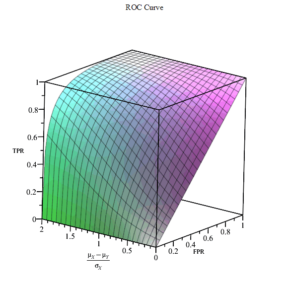
Assuming that a = `/`(`*`(`+`(mu__X, `-`(mu__Y))), `*`(sigma__X)); -1and that b = `/`(`*`(sigma__Y), `*`(sigma__X)); -1we can compute the ROC curve for two normal distributions as follows: 

R := proc (a, b, t) options operator, arrow, function_assign; Phi(`+`(a, `*`(b, `*`(Q(t))))) end proc; 1 

Typesetting:-mprintslash([R := proc (a, b, t) options operator, arrow, function_assign; Phi(`+`(a, `*`(b, `*`(Q(t))))) end proc], [proc (a, b, t) options operator, arrow, function_assign; Phi(`+`(a, `... (1.3)
 

plot3d(R(a, 1, t), t = 0 .. 1, a = 0 .. 2, labels = [ 

Plot_2d
 

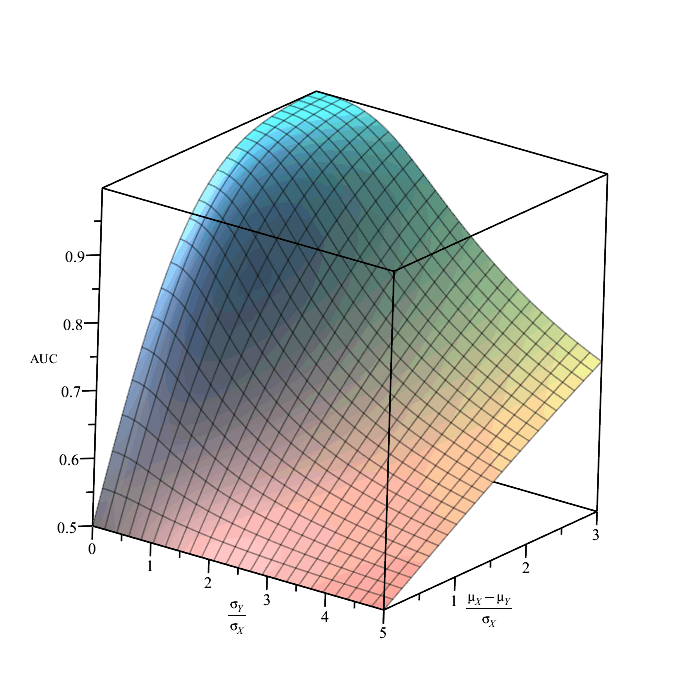
The area under the ROC curve (AUC) can be computed as follows: 

AUC := proc (a, b) options operator, arrow, function_assign; Phi(`/`(`*`(a), `*`(sqrt(`+`(1, `*`(`^`(b, 2))))))) end proc; 1 

Typesetting:-mprintslash([AUC := proc (a, b) options operator, arrow, function_assign; Phi(`/`(`*`(a), `*`(sqrt(`+`(1, `*`(`^`(b, 2))))))) end proc], [proc (a, b) options operator, arrow, function_ass... (1.4)
 

plot3d(AUC(a, b), b = 0 .. 5, a = 0 .. 3, labels = ['`/`(`*`(sigma__Y), `*`(sigma__X))', '`/`(`*`(`+`(mu__X, `-`(mu__Y))), `*`(sigma__X))',  

Plot_2d
 

The U-statistic for the binormal model with sample sizes N__X; and N__Y; can be computed from the AUC as follows:  

U := proc (a, b, N__X, N__Y) options operator, arrow, function_assign; `*`(AUC(a, b), `*`(N__X, `*`(N__Y))) end proc; 1 

Typesetting:-mprintslash([U := proc (a, b, N__X, N__Y) options operator, arrow, function_assign; `*`(AUC(a, b), `*`(N__X, `*`(N__Y))) end proc], [proc (a, b, N__X, N__Y) options operator, arrow, funct... (1.5)


Computing P-Values from the U-Statistic 

At large samples, the U-statistic is normally distributed with mean 

M__U := proc (N__X, N__Y) options operator, arrow, function_assign; `+`(`*`(`/`(1, 2), `*`(N__Y, `*`(N__X)))) end proc; 1 

Typesetting:-mprintslash([M__U := proc (N__X, N__Y) options operator, arrow, function_assign; `+`(`*`(`/`(1, 2), `*`(N__Y, `*`(N__X)))) end proc], [proc (N__X, N__Y) options operator, arrow, function_... (2.1)
 

and the standard deviation is  

s__U := proc (N__X, N__Y) options operator, arrow, function_assign; sqrt(`+`(`*`(`/`(1, 12), `*`(N__X, `*`(N__Y(`+`(N__X, N__Y, 1))))))) end proc; 1 

Typesetting:-mprintslash([s__U := proc (N__X, N__Y) options operator, arrow, function_assign; sqrt(`+`(`*`(`/`(1, 12), `*`(N__X, `*`(N__Y(`+`(N__X, N__Y, 1))))))) end proc], [proc (N__X, N__Y) options... (2.2)
 

We can therefore compute a Z-score: 

Z := proc (a, b, N__X, N__Y) options operator, arrow, function_assign; `/`(`*`(`+`(U(a, b, N__X, N__Y), `-`(M__U(N__X, N__Y)))), `*`(s__U(N__X, N__Y))) end proc; 1 

Typesetting:-mprintslash([Z := proc (a, b, N__X, N__Y) options operator, arrow, function_assign; `/`(`*`(`+`(U(a, b, N__X, N__Y), `-`(M__U(N__X, N__Y)))), `*`(s__U(N__X, N__Y))) end proc], [proc (a, b... (2.3)
 

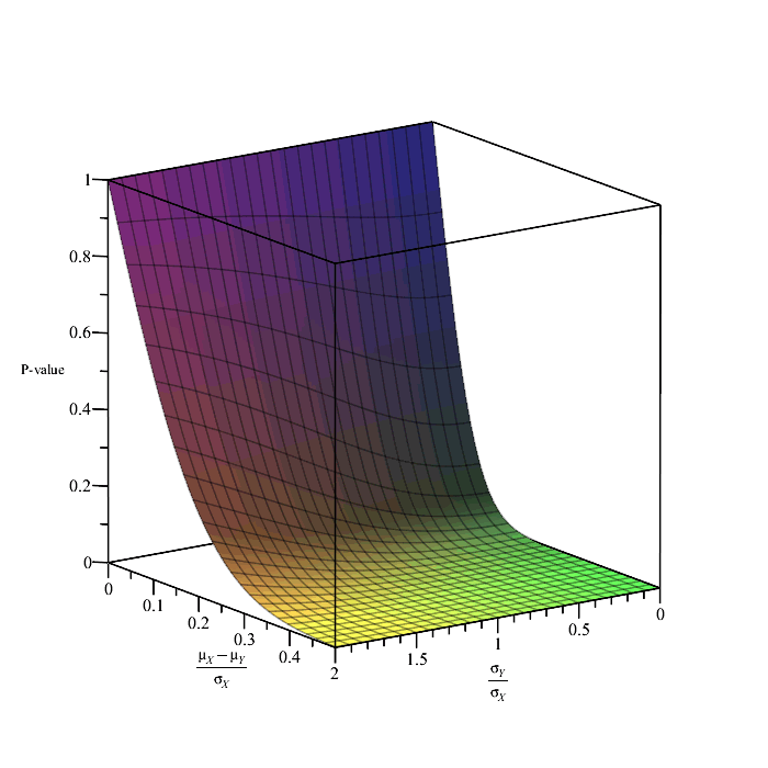
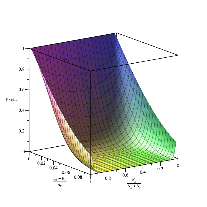
A two-tailed p-value is thus 

P := proc (a, b, N__X, N__Y) options operator, arrow, function_assign; `+`(2, `-`(`*`(2, `*`(Phi(abs(Z(a, b, N__X, N__Y))))))) end proc;  

Typesetting:-mprintslash([P := proc (a, b, N__X, N__Y) options operator, arrow, function_assign; `+`(2, `-`(`*`(2, `*`(Phi(abs(Z(a, b, N__X, N__Y))))))) end proc], [proc (a, b, N__X, N__Y) options ope... (2.4)
 

plot3d(P(a, b, 10, 10), b = 0 .. 2, a = 0 .. .5, labels = ['`/`(`*`(sigma__Y), `*`(sigma__X))', '`/`(`*`(`+`(mu__X, `-`(mu__Y))), `*`(sigma__X))',  

Plot_2d
 

plot3d(P(a, 1, `+`(`*`(100, `*`(c))), `+`(100, `-`(`*`(100, `*`(c))))), c = 0 .. 1, a = 0 .. .1, labels = [`/`(`*`(N__X), `*`(`+`(N__X, N__Y))), '`/`(`*`(`+`(mu__X, `-`(mu__Y))), `*`(sigma__X))',  

Plot_2d